Understanding Big O

How efficient is your algorithm?

It’s indispensable to have a clear understanding of basic algorithms before attending a programming interview. In order to understand algorithms, it’s also important to know to measure the efficiency of an algorithm. This is done with a concept, called the Big O. There exists a common question that pops up on an algorithm interview as to “How efficient is your algorithm?”. So, unless you can come up with this from scratch and measure it, rather than memorizing it for different problems, it may cause your interview to drift away from a successful one.

In this article, we’ll try to simplify the understanding of the concept of Big O which may help you prepare for a programming interview or understanding how you can use it. We will try to understand Big O from first principles rather than encouraging ourselves to memorize the Big O for different problems. I will use the Python programming language for all the examples in this article.

What is Big O for?

Big O is a concept critical to algorithms and the most mathematical we’ll get in this article. Two main reasons of understanding this concept are:

1. If you get a problem that you haven’t seen before, although you have experience dealing with hundreds of problems before, there’s a chance that you end up with one problem that you have never come across, and hence you’ll not know how to get the Big O.
2. In an interview, you may get partial or almost full credit to show your work on getting the Big O although your exact answer may not be correct.

In reality, programming interviews focus mainly on your problem-solving abilities, which definitely comes down to breaking down your algorithm and explaining step-by-step what you think your Big O might be.

What is Big O?

Big O represents the efficiency of your algorithm and is of two different types:

1. Time-based — related to performance, speed, and in turn efficiency of the code;
2. Space-based — related to memory, in turn relating to how much extra space for variables and data structures are required to solve the algorithm.

Therefore, if you have large inputs for your functions within your algorithm, both time and space will start to cause problems. Hence the relevance of these to types for Big O. These types are also often used as a benchmark to compare different algorithms and measure how good they are. For example, there are a lot of different ways a code sort, and they all have different efficiencies. So, this is a measure of grading these efficiencies, just like the grading system in academics.

Now let’s look at how exactly we assign this grade. This is done, not in absolute terms, but in terms relative to the size of the input. Consider an input as an argument to a function. Now, if we double the size of this input, we check if the time and space scale up proportionally, slightly less, or slightly more.

Consider a function called length(input) that measures the length of an array or of a string. Now we can pass in the input of size 3 and say that it takes 1 full second to complete (not a great one, but consider for the sake of our example). And next let’s pass in an array of size 6 and say it takes 2 full seconds to complete.

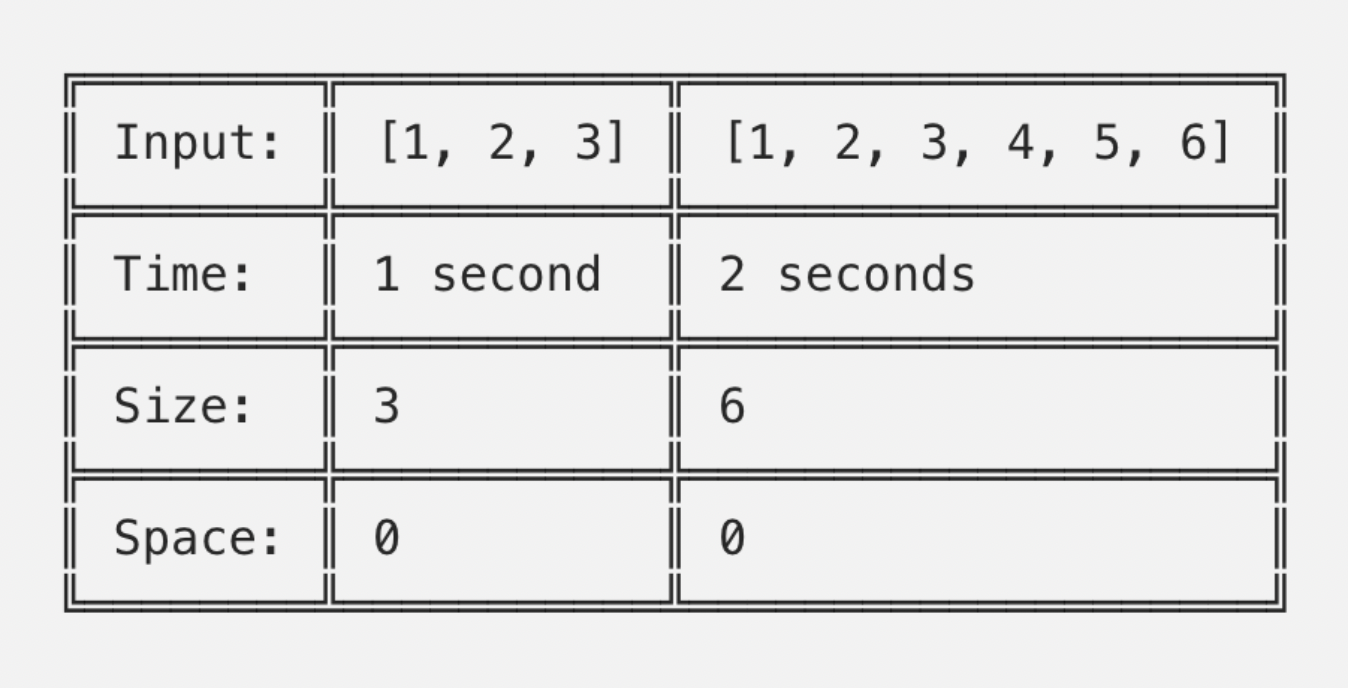
When comparing the inputs and their times, we can observe that doubling the input size, doubles the execution time. This proportional increase in time is known as linear time. In other words, the relationship between time and input in our example is 1:1. In Big O notation, we call this linear time “O” of “n”, written as O(n). Note that in this example we did not use any extra space.

Extra space does not include the size of our input, so we start and end with zero space. If either space or the time has no relationship with the input, we call it constant space and in Big O notations, we designate it as O(1). These terms are referred to as order with each being a different tier of efficiency. The below list shows the order of most efficient (or shortest time or the least space) to the least efficient Big O’s.

1. O(1) — constant
2. O(log n) — logarithmic
3. O(n) — linear
4. O(n log n) — linear * log
5. O(n * n) — quadratic
6. O(2^ n) — exponential

Now let’s take a look at what’s inside our length(input) function:

def length(input):
  counter = 0
  for i in input:
      counter += 1
  return counter

Observe the counter variable and the loop in the code. In reality, every single line of code has its own time complexity, but using little tricks, you can get the line’s time complexity reduced. The key is in the question — How does the input size, whether it’s string length or array length, affect this specific line?

If the answer comes down to the fact that it does not have a direct impact, then by default, that line is constant time, simply because it has no relationship to the input. Looking at our first line of the code (counter = 0), note that creating the counter variable is going to happen whether we pass 1 or 100 array items. Therefore, by default, this line is constant time. Next, consider asking if the counter variable is a constant space or does this variable scale with the size of our input. The usual assumption would be yes, since we’re incrementing the counter up to the length of our input. However, the truth is integers always take up the same amount of space unless they’re really large numbers. So, once we have identified that the first line is constant, we shift our focus on the loop. Notice that this will run n-times proportional to the size of our input. Hence there is a direct relationship between our input and the time of this line of our code. Now in order to find the relationship, simply take two different inputs. For example, take an input of array size 1 versus an array of size 2: [1] vs [1, 2]

So, we need 1 iteration for array of size 1 and 2 iterations for an array of size 2. Clearly, there is a one-to-one relationship, hence, linear O(n).

Now if we want to determine the time-complexity, notice that we have O(1) for counter initialization and then O(n) for the loop. Therefore, we can say that it is taking O(1) + O(n) time altogether. Observe that even in this very simple function, we have multiple terms. Needless to say, for longer functions, we have many multiple complex additions of time complexities. This is a very hideous task, and so, we need to simplify. This simplification is done by only keeping the terms that are in the highest order. So in our example, we will end up dropping the O(1) for counter initialization, since relative to O(n) its effects are negligible. Since each tier of Big O is an order of magnitude larger than the ones below it, when we get to larger size inputs, the lower order terms become completely irrelevant. So for our example, if we have O(300), it would be absolutely negligible compared to our n=300. In case we had O(n * n) then we would have O(90000) which will then make n=300 totally negligible.

To sum up, simplification includes:

1. Dropping the lower order terms, and
2. Dropping the constant terms.

Consider another example with two loops now:

def sumAndLength(input):
    sum = 0
    length = 0
    for num in input:
        sum += num
    for i in input:
        length += 1
    return (sum, length)

Now we have two O(n), one for the first loop, and one for the second loop.

Here we have n + n = 2n (in practice, we can simply drop the coefficient “2” since all we are concerned about is the order). This is because the orders are so large compared to each other, that the presence or absence of the coefficients (whether 2n, or 4n, or 100n compared to n*n).

This is how we simplify Big O for our algorithms. The length(input) function that we used was a nice clean example since we always increment the counter n times, 1 for each iteration of the loop.

In most cases, however, functions have a range of efficiencies rather than an exact value. This can be made clear with an example. Let’s say we’re using the find function as below:

index = 'qwerty'.find('w')

This function searches for a string or a character and returns its index upon finding the substring and otherwise returns -1 if the substring is not found.

To consider using Big O, we must train ourselves to think about the entire spectrum of possibilities. Most importantly, we should determine the best case with the least amount of effort or the worst case with the most amount of effort.

def index(input, target):
  for i, char in enumerate(input):
    if char == target:
      return i
    return -1

So, for the index function, it searches the string for a target character one at a time, and then once found, it returns its index. In this case, we should train ourselves to consider both:

1. Best-case scenario, i.e. the character is found at the beginning of the input string;
2. Worst-case scenario, i.e. the character is not found within the input string.

Therefore we conclude that our best case is O(1) (since it’s a single iteration leading to a single operation) and our worst case is O(n) (since the input now is proportional to the length of our entire string). With Big O, it’s a convention to always take the worst case, and hence for this case, we can say that the index function is O(n) or linear time.

Conclusion

So, these are the basics of understanding how Big O can be beneficial in determining the efficiency of your algorithm. To sum up, the take away from our reading are the following:

• Every line of code has a Big O time complexity;
• Every variable we create has a space complexity;
• We simplify the Big O sums by considering only the highest order of terms;
• Constants are dropped to recognize the order and simplify further;
• When scanning through the entire spectrum of possible inputs, we always consider the worst-case scenario.

When comparing the inputs and their times, we can observe that doubling the input size, doubles the execution time. This proportional increase in time is known as linear time. In other words, the relationship between time and input in our example is 1:1. In Big O notation, we call this linear time “O” of “n”, written as O(n). Note that in this example we did not use any extra space.